Configuration Space

Chapter 2

Configuration Space

A robot is mechanically constructed by connecting a set of bodies, called links, to each other using various types of joints. Actuators, such as electric motors, deliver forces or torques that cause the robot's links to move. Usually an end- effector, such as a gripper or hand for grasping and manipulating objects, is attached to a specific link. All the robots considered in this book have links that can be modeled as rigid bodies.

Perhaps the most fundamental question one can ask about a robot is, where is it? The answer is given by the robot's configuration: a specification of the positions of all points of the robot. Since the robot's links are rigid and of a known shape, 1 only a few numbers are needed to represent its configuration. For example, the configuration of a door can be represented by a single number, the angle θ about its hinge. The configuration of a point on a plane can be described by two coordinates, (x,y) . The configuration of a coin lying heads up on a flat table can be described by three coordinates: two coordinates (x,y) that specify the location of a particular point on the coin, and one coordinate (θ) that specifies the coin's orientation. (See Figure 2.1).

The above coordinates all take values over a continuous range of real numbers. The number of degrees of freedom (dof) of a robot is the smallest number of real- valued coordinates needed to represent its configuration. In the example above, the door has one degree of freedom. The coin lying heads up on a table has three degrees of freedom. Even if the coin could lie either heads up or tails up, its configuration space still would have only three degrees of freedom; a fourth variable, representing which side of the coin faces up, takes values in the discrete set {heads, tails}, and not over a continuous range of real

<--- Page 57 --->

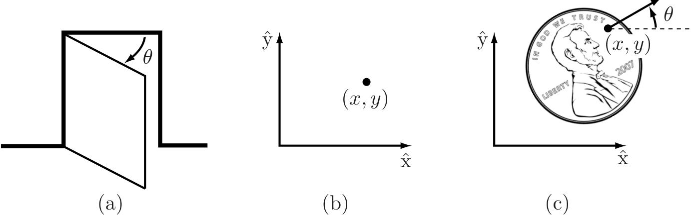
Figure 2.1: (a) The configuration of a door is described by the angle $\theta$ . (b) The configuration of a point in a plane is described by coordinates $(x, y)$ . (c) The configuration of a coin on a table is described by $(x, y,\theta)$ , where $\theta$ defines the direction in which Abraham Lincoln is looking.

values like the other three coordinates.

Definition 2.1. The configuration of a robot is a complete specification of the position of every point of the robot. The minimum number n of real- valued coordinates needed to represent the configuration is the number of degrees of freedom (dof) of the robot. The n - dimensional space containing all possible configurations of the robot is called the configuration space (C- space). The configuration of a robot is represented by a point in its C- space.

In this chapter we study the C- space and degrees of freedom of general robots. Since our robots are constructed from rigid links, we examine first the degrees of freedom of a single rigid body, and then the degrees of freedom of general multi- link robots. Next we study the shape (or topology) and geometry of C- spaces and their mathematical representation. The chapter concludes with a discussion of the C- space of a robot's end- effector, its task space. In the following chapter we study in more detail the mathematical representation of the C- space of a single rigid body.

2.1 Degrees of Freedom of a Rigid Body

Continuing with the example of the coin lying on the table, choose three points A , B , and C on the coin (Figure 2.2 (a)). Once a coordinate frame x^y^ is attached to the plane, the positions of these points in the plane are written

<--- Page 57 --->

Figure 2.2: (a) Choosing three points fixed to the coin. (b) Once the location of $A$ is chosen, $B$ must lie on a circle of radius $d_{AB}$ centered at $A$ . Once the location of $B$ is chosen, $C$ must lie at the intersection of circles centered at $A$ and $B$ . Only one of these two intersections corresponds to the “heads up” configuration. (c) The configuration of a coin in three-dimensional space is given by the three coordinates of $A$ , two angles to the point $B$ on the sphere of radius $d_{AB}$ centered at $A$ , and one angle to the point $C$ on the circle defined by the intersection of the a sphere centered at $A$ and a sphere centered at $B$ .

(xA,yA) (xB,yB) ,and (xC,yC) . If the points could be placed independently anywhere in the plane, the coin would have six degrees of freedom - two for each of the three points. But, according to the definition of a rigid body, the distance between point A and point B , denoted d(A,B) , is always constant regardless of where the coin is. Similarly, the distances d(B,C) and d(A,C) must be constant. The following equality constraints on the coordinates (xA,yA) (xB,yB) ,and (xC,yC) must therefore always be satisfied:

d(A,B)=(xAxB)2+(yAyB)2=dAB,$$$$d(B,C)=(xBxC)2+(yByC)2=dBC,$$$$d(A,C)=(xAxC)2+(yAyC)2=dAC.

To determine the number of degrees of freedom of the coin on the table, first choose the position of point A in the plane (Figure 2.2 (b)). We may choose it to be anything we want, so we have two degrees of freedom to specify, namely (xA,yA) . Once (xA,yA) is specified, the constraint d(A,B)=dAB restricts the choice of (xB,yB) to those points on the circle of radius dAB centered at A . A point on this circle can be specified by a single parameter, e.g., the angle specifying the location of B on the circle centered at A . Let's call this angle ϕAB and define it to be the angle that the vector AB makes with the x^ - axis.

<--- Page 57 --->

Once we have chosen the location of point B , there are only two possible locations for C : at the intersections of the circle of radius dAC centered at A and the circle of radius dBC centered at B (Figure 2.2 (b)). These two solutions correspond to heads or tails. In other words, once we have placed A and B and chosen heads or tails, the two constraints d(A,C)=dAC and d(B,C)=dBC eliminate the two apparent freedoms provided by (xC,yC) , and the location of C is fixed. The coin has exactly three degrees of freedom in the plane, which can be specified by (xA,yA,ϕAB) .

Suppose that we choose to specify the position of an additional point D on the coin. This introduces three additional constraints: d(A,D)=dAD , d(B,D)=dBD , and d(C,D)=dCD . One of these constraints is redundant, i.e., it provides no new information; only two of the three constraints are independent. The two freedoms apparently introduced by the coordinates (xD,yD) are then immediately eliminated by these two independent constraints. The same would hold for any other newly chosen point on the coin, so that there is no need to consider additional points.

We have been applying the following general rule for determining the number of degrees of freedom of a system:

degrees of freedom=(sum of freedoms of the points)(2.1)

This rule can also be expressed in terms of the number of variables and independent equations that describe the system:

degrees of freedom=(number of variables)(number of independent equations).(2.2)

This general rule can also be used to determine the number of freedoms of a rigid body in three dimensions. For example, assume our coin is no longer confined to the table (Figure 2.2 (c)). The coordinates for the three points A,B , and C are now given by (xA,yA,zA) , (xB,yB,zB) , and (xC,yC,zC) , respectively. Point A can be placed freely (three degrees of freedom). The location of point B is subject to the constraint d(A,B)=dAB , meaning it must lie on the sphere of radius dAB centered at A . Thus we have 31=2 freedoms to specify, which can be expressed as the latitude and longitude for the point on the sphere. Finally, the location of point C must lie at the intersection of spheres centered at A and B of radius dAC and dBC , respectively. In the general case the intersection of two spheres is a circle, and the location of point C can be described by an angle that parametrizes this circle. Point C therefore adds 32=1 freedom. Once the position of point C is chosen, the coin is fixed in space.

<--- Page 57 --->

In summary, a rigid body in three- dimensional space has six freedoms, which can be described by the three coordinates parametrizing point A , the two angles parametrizing point B , and one angle parametrizing point C , provided A , B , and C are noncollinear. Other representations for the configuration of a rigid body are discussed in Chapter 3.

We have just established that a rigid body moving in three- dimensional space, which we call a spatial rigid body, has six degrees of freedom. Similarly, a rigid body moving in a two- dimensional plane, which we henceforth call a planar rigid body, has three degrees of freedom. This latter result can also be obtained by considering the planar rigid body to be a spatial rigid body with six degrees of freedom but with the three independent constraints zA=zB=zC=0 .

Since our robots consist of rigid bodies, Equation (2.1) can be expressed as follows:

degrees of freedom=(sum of freedoms of the bodies)$$$$(number of independent constraints).

Equation (2.3) forms the basis for determining the degrees of freedom of general robots, which is the topic of the next section.

2.2 Degrees of Freedom of a Robot

Consider once again the door example of Figure 2.1 (a), consisting of a single rigid body connected to a wall by a hinge joint. From the previous section we know that the door has only one degree of freedom, conveniently represented by the hinge joint angle θ . Without the hinge joint, the door would be free to move in three- dimensional space and would have six degrees of freedom. By connecting the door to the wall via the hinge joint, five independent constraints are imposed on the motion of the door, leaving only one independent coordinate (θ) . Alternatively, the door can be viewed from above and regarded as a planar body, which has three degrees of freedom. The hinge joint then imposes two independent constraints, again leaving only one independent coordinate (θ) . The door's C- space is represented by some range in the interval [0,2π) over which θ is allowed to vary.

In both cases the joints constrain the motion of the rigid body, thus reducing the overall degrees of freedom. This observation suggests a formula for determining the number of degrees of freedom of a robot, simply by counting the number of rigid bodies and joints. In this section we derive precisely such

<--- Page 57 --->

Figure 2.3: Typical robot joints.

a formula, called Grübler's formula, for determining the number of degrees of freedom of planar and spatial robots.

2.2.1 Robot Joints

Figure 2.3 illustrates the basic joints found in typical robots. Every joint connects exactly two links; joints that simultaneously connect three or more links are not allowed. The revolute joint (R), also called a hinge joint, allows rotational motion about the joint axis. The prismatic joint (P), also called a sliding or linear joint, allows translational (or rectilinear) motion along the direction of the joint axis. The helical joint (H), also called a screw joint, allows simultaneous rotation and translation about a screw axis. Revolute, prismatic, and helical joints all have one degree of freedom.

Joints can also have multiple degrees of freedom. The cylindrical joint (C) has two degrees of freedom and allows independent translations and rotations about a single fixed joint axis. The universal joint (U) is another two- degreeof- freedom joint that consists of a pair of revolute joints arranged so that their joint axes are orthogonal. The spherical joint (S), also called a ball- and- socket joint, has three degrees of freedom and functions much like our shoulder joint.

A joint can be viewed as providing freedoms to allow one rigid body to move relative to another. It can also be viewed as providing constraints on the possible motions of the two rigid bodies it connects. For example, a revolute joint can be viewed as allowing one freedom of motion between two rigid bodies

<--- Page 57 --->

Joint typedof fConstraints c between two planar rigid bodiesConstraints c between two spatial rigid bodies
Revolute (R)125
Prismatic (P)125
Helical (H)1N/A5
Cylindrical (C)2N/A4
Universal (U)2N/A4
Spherical (S)3N/A3

Table 2.1: The number of degrees of freedom f and constraints c provided by common joints.

in space, or it can be viewed as providing five constraints on the motion of one rigid body relative to the other. Generalizing, the number of degrees of freedom of a rigid body (three for planar bodies and six for spatial bodies) minus the number of constraints provided by a joint must equal the number of freedoms provided by that joint.

The freedoms and constraints provided by the various joint types are summarized in Table 2.1.

2.2.2 Grübler's Formula

The number of degrees of freedom of a mechanism with links and joints can be calculated using Grübler's formula, which is an expression of Equation (2.3).

Proposition 2.2. Consider a mechanism consisting of N links, where ground is also regarded as a link. Let J be the number of joints, m be the number of degrees of freedom of a rigid body (m=3 for planar mechanisms and m=6 for spatial mechanisms), fi be the number of freedoms provided by joint i, and ci be the number of constraints provided by joint i, where fi+ci=m for all i. Then

<--- Page 57 --->

Figure 2.4: (a) Four-bar linkage. (b) Slider-crank mechanism.

Gribler's formula for the number of degrees of freedom of the robot is

df=m(N1)rigid body freedomsi=1Jcijoint constraints=m(N1)i=1J(mfi)=m(N1J)+i=1Jfi.(2.4)

This formula holds in "generic" cases, but it fails under certain configurations of the links and joints, such as when the joint constraints are not independent.

Below we apply Gribler's formula to several planar and spatial mechanisms. We distinguish between two types of mechanism: open- chain mechanisms. (also known as serial mechanisms) and closed- chain mechanisms. A closed- chain mechanism is any mechanism that has a closed loop. A person standing with both feet on the ground is an example of a closed- chain mechanism, since a closed loop can be traced from the ground, through the right leg, through the waist, through the left leg, and back to ground (recall that the ground itself is a link). An open- chain mechanism is any mechanism without a closed loop; an example is your arm when your hand is allowed to move freely in space.

Example 2.3 (Four- bar linkage and slider- crank mechanism). The planar fourbar linkage shown in Figure 2.4 (a) consists of four links (one of them ground) arranged in a single closed loop and connected by four revolute joints. Since all the links are confined to move in the same plane, we have m=3 . Substituting N=4 , J=4 , and fi=1 , i=1,,4 , into Gribler's formula, we see that the four- bar linkage has one degree of freedom.

<--- Page 57 --->

Figure 2.5: (a) k - link planar serial chain. (b) Five- bar planar linkage. (c) Stephenson six- bar linkage. (d) Watt six- bar linkage.

The slider- crank closed- chain mechanism of Figure 2.4 (b) can be analyzed in two ways: (i) the mechanism consists of three revolute joints and one prismatic joint (J=4 and each fi=1) ) and four links (N=4 , including the ground link), or (ii) the mechanism consists of two revolute joints (fi=1) ) and one RP joint (the RP joint is a concatenation of a revolute and prismatic joint, so that fi=2 ) and three links (N=3 ; remember that each joint connects precisely two bodies). In both cases the mechanism has one degree of freedom.

Example 2.4 (Some classical planar mechanisms). Let us now apply Grübler's formula to several classical planar mechanisms. The k - link planar serial chain of revolute joints in Figure 2.5 (a) (called a kR robot for its k revolute joints) has N=k+1 links ( k links plus ground), and J=k joints, and, since all the joints are revolute, fi=1 for all i . Therefore,

dof=3((k+1)1k)+k=k

<--- Page 57 --->

Figure 2.6: A planar mechanism with two overlapping joints.

as expected. For the planar five- bar linkage of Figure 2.5 (b), N=5 (four links plus ground), J=5, and since all joints are revolute, each fi=1. Therefore,

dof=3(515)+5=2.

For the Stephenson six- bar linkage of Figure 2.5 (c), we have N=6 , J=7, and fi=1 for all i, so that

dof=3(617)+7=1.

Finally, for the Watt six- bar linkage of Figure 2.5 (d), we have N=6 , J=7, and fi=1 for all i, so that, like the Stephenson six- bar linkage,

dof=3(617)+7=1.

Example 2.5 (A planar mechanism with overlapping joints). The planar mechanism illustrated in Figure 2.6 has three links that meet at a single point on the right of the large link. Recalling that a joint by definition connects exactly two links, the joint at this point of intersection should not be regarded as a single revolute joint. Rather, it is correctly interpreted as two revolute joints overlapping each other. Again, there is more than one way to derive the number of degrees of freedom of this mechanism using Grübler's formula: (i) The mechanism consists of eight links (N=8) , eight revolute joints, and one prismatic joint. Substituting into Grübler's formula yields

dof=3(819)+9(1)=3.

(ii) Alternatively, the lower- right revolute–prismatic joint pair can be regarded as a single two- dof joint. In this case the number of links is N=7, with seven

<--- Page 57 --->

Figure 2.7: (a) A parallelogram linkage. (b) The five-bar linkage in a regular and singular configuration.

revolute joints, and a single two- dof revolute- prismatic pair. Substituting into Grübler's formula yields

dof=3(718)+7(1)+1(2)=3.

Example 2.6 (Redundant constraints and singularities). For the parallelogram linkage of Figure 2.7 (a), N=5 , J=6 , and fi=1 for each joint. From Grübler's formula, the number of degrees of freedom is 3(516)+6=0 . A mechanism with zero degrees of freedom is by definition a rigid structure. It is clear from examining the figure, though, that the mechanism can in fact move with one degree of freedom. Indeed, any one of the three parallel links, with its two joints, has no effect on the motion of the mechanism, so we should have calculated dof=3(414)+4=1 . In other words, the constraints provided by the joints are not independent, as required by Grübler's formula.

A similar situation arises for the two- dof planar five- bar linkage of Figure 2.7 (b). If the two joints connected to ground are locked at some fixed angle, the five- bar linkage should then become a rigid structure. However, if the two middle links are the same length and overlap each other, as illustrated in Figure 2.7 (b), these overlapping links can rotate freely about the two overlapping joints. Of course, the link lengths of the five- bar linkage must meet certain specifications in order for such a configuration to even be possible. Also note that if a different pair of joints is locked in place, the mechanism does become a rigid structure as expected.

Example 2.7 (Delta robot). The Delta robot of Figure 2.8 consists of two platforms – the lower one mobile, the upper one stationary – connected by three legs. Each leg contains a parallelogram closed chain and consists of three revolute joints, four spherical joints, and five links. Adding the two platforms,

<--- Page 57 --->

Figure 2.8: The Delta robot.

there are N=17 links and J=21 joints (nine revolute and 12 spherical). By Grübler's formula,

df=6(17121)+9(1)+12(3)=15.

Of these 15 degrees of freedom, however, only three are visible at the end- . effector on the moving platform. In fact, the parallelogram leg design ensures that the moving platform always remains parallel to the fixed platform, so that the Delta robot acts as an xyz Cartesian positioning device. The other 12 internal degrees of freedom are accounted for by torsion of the 12 links in the parallelograms (each of the three legs has four links in its parallelogram) about their long axes..

Example 2.8 (Stewart–Gough platform). The Stewart–Gough platform of Figure 1.1 (b) consists of two platforms – the lower one stationary and regarded as ground, the upper one mobile – connected by six universal– prismatic–spherical (UPS) legs. The total number of links is 14 (N=14) . There are six universal joints (each with two degrees of freedom, fi=2 ), six prismatic joints (each with a single degree of freedom, fi=1 ), and six spherical joints (each with three degrees of freedom, fi=3 ). The total number of joints is 18. Substituting these values into Grübler’s formula with m=6 yields

df=6(14118)+6(1)+6(2)+6(3)=6.

<--- Page 57 --->

In some versions of the Stewart- Gough platform the six universal joints are replaced by spherical joints. By Grübler's formula this mechanism has 12 degrees of freedom; replacing each universal joint by a spherical joint introduces an extra degree of freedom in each leg, allowing torsional rotations about the leg axis. Note, however, that this torsional rotation has no effect on the motion of the mobile platform.

The Stewart- Gough platform is a popular choice for car and airplane cockpit simulators, as the platform moves with the full six degrees of freedom of motion of a rigid body. On the one hand, the parallel structure means that each leg needs to support only a fraction of the weight of the payload. On the other hand, this structure also limits the range of translational and rotational motion of the platform relative to the range of motion of the end- effector of a six- dof open chain.

2.3 Configuration Space: Topology and Representation

2.3.1 Configuration Space Topology

Until now we have been focusing on one important aspect of a robot’s C- space – its dimension, or the number of degrees of freedom. However, the shape of the space is also important.

Consider a point moving on the surface of a sphere. The point’s C- space is two dimensional, as the configuration can be described by two coordinates, latitude and longitude. As another example, a point moving on a plane also has a two- dimensional C- space, with coordinates (x,y) . While both a plane and the surface of a sphere are two dimensional, clearly they do not have the same shape – the plane extends infinitely while the sphere wraps around.

Unlike the plane, a larger sphere has the same shape as the original sphere, in that it wraps around in the same way. Only its size is different. For that matter, an oval- shaped American football also wraps around similarly to a sphere. The only difference between a football and a sphere is that the football has been stretched in one direction.

The idea that the two- dimensional surfaces of a small sphere, a large sphere, and a football all have the same kind of shape, which is different from the shape of a plane, is expressed by the topology of the surfaces. We do not attempt a rigorous treatment in this book,3 but we say that two spaces are topologically

<--- Page 57 --->

Figure 2.9: An open interval of the real line, denoted $(a, b)$ , can be deformed to an open semicircle. This open semicircle can then be deformed to the real line by the mapping illustrated: beginning from a point at the center of the semicircle, draw a ray that intersects the semicircle and then a line above the semicircle. These rays show that every point of the semicircle can be stretched to exactly one point on the line, and vice versa. Thus an open interval can be continuously deformed to a line, so an open interval and a line are topologically equivalent.

equivalent if one can be continuously deformed into the other without cutting or gluing. A sphere can be deformed into a football simply by stretching, without cutting or gluing, so those two spaces are topologically equivalent. You cannot turn a sphere into a plane without cutting it, however, so a sphere and a plane are not topologically equivalent.

Topologically distinct one- dimensional spaces include the circle, the line, and a closed interval of the line. The circle is written mathematically as S or S1 , a one- dimensional "sphere." The line can be written as E or E1 , indicating a one- dimensional Euclidean (or "flat") space. Since a point in E1 is usually represented by a real number (after choosing an origin and a length scale), it is often written as R or R1 instead. A closed interval of the line, which contains its endpoints, can be written [a,b]R1 . (An open interval (a,b) does not include the endpoints a and b and is topologically equivalent to a line, since the open interval can be stretched to a line, as shown in Figure 2.9. A closed interval is not topologically equivalent to a line, since a line does not contain endpoints.)

In higher dimensions, Rn is the n - dimensional Euclidean space and Sn is the n - dimensional surface of a sphere in (n+1) - dimensional space. For example, S2 is the two- dimensional surface of a sphere in three- dimensional space.

Note that the topology of a space is a fundamental property of the space itself and is independent of how we choose coordinates to represent points in the space. For example, to represent a point on a circle, we could refer to the point by the angle θ from the center of the circle to the point, relative to a chosen zero angle. Or, we could choose a reference frame with its origin at the center of the circle and represent the point by the two coordinates (x,y) subject to the constraint x2+y2=1 . No matter what our choice of coordinates is, the space itself does not change.

Some C- spaces can be expressed as the Cartesian product of two or more space.

<--- Page 57 --->

spaces of lower dimension; that is, points in such a C- space can be represented as the union of the representations of points in the lower-dimensional spaces. For example:

The C- space of a rigid body in the plane can be written as R2×S1 , since the configuration can be represented as the concatenation of the coordinates (x,y) representing R2 and an angle θ representing S1 .

The C- space of a PR robot arm can be written R1×S1 . (We will occasionally ignore joint limits, i.e., bounds on the travel of the joints, when expressing the topology of the C- space; with joint limits, the C- space is the Cartesian product of two closed intervals of the line.)

The C- space of a 2R robot arm can be written S1×S1=T2 , where Tn is the n - dimensional surface of a torus in an (n+1) - dimensional space. (See Table 2.2. ) Note that S1×S1××S1 ( n copies of S1 ) is equal to Tn , not Sn ; for example, a sphere S2 is not topologically equivalent to a torus T2 .

The C- space of a planar rigid body (e.g., the chassis of a mobile robot) with a 2R robot arm can be written as R2×S1×T2=R2×T3 .

As we saw in Section 2.1 when we counted the degrees of freedom of a rigid body in three dimensions, the configuration of a rigid body can be described by a point in R3 , plus a point on a two- dimensional sphere S2 , plus a point on a one- dimensional circle S1 , giving a total C- space of R3×S2×S1 .

2.3.2 Configuration Space Representation

To perform computations, we must have a numerical representation of the space, consisting of a set of real numbers. We are familiar with this idea from linear algebra – a vector is a natural way to represent a point in a Euclidean space. It is important to keep in mind that the representation of a space involves a choice, and therefore it is not as fundamental as the topology of the space, which is independent of the representation. For example, the same point in a three- dimensional space can have different coordinate representations depending on the choice of reference frame (the origin and the direction of the coordinate axes) and the choice of length scale, but the topology of the underlying space is the same regardless of these choices.

While it is natural to choose a reference frame and length scale and to use a vector to represent points in a Euclidean space, representing a point on a

<--- Page 57 --->

systemtopologysample representation
point on a planeE2(x, y)
R2
spherical pendulumS2latitude
90°
-180° -90°
[-180°, 180°) × [-90°, 90°]
2R robot armT2=S1×S1θ2

[0,2π)×[0,2π)
rotating sliding knobE1×S1θ

R1×[0,2π)

Table 2.2: Four topologically different two-dimensional C-spaces and example co-ordinate representations. In the latitude-longitude representation of the sphere, the latitudes 90 and 90 each correspond to a single point (the South Pole and the North Pole, respectively), and the longitude parameter wraps around at 180 and 180; the edges with the arrows are glued together. Similarly, the coordinate representations of the torus and cylinder wrap around at the edges marked with corresponding arrows.

curved space, such as a sphere, is less obvious. One solution for a sphere is to use latitude and longitude coordinates. A choice of n coordinates, or parameters,

<--- Page 57 --->

to represent an n - dimensional space is called an explicit parametrization of the space. Such an explicit parametrization is valid for a particular range of the parameters (e.g., [90,90] for latitude and [180,180) for longitude for a sphere, where, on Earth, negative values correspond to "south" and "west," respectively).

The latitude- longitude representation of a sphere is unsatisfactory if you are walking near the North Pole (where the latitude equals 90 ) or South Pole (where the latitude equals 90 ), where taking a very small step can result in a large change in the coordinates. The North and South Poles are singularities of the representation, and the existence of singularities is a result of the fact that a sphere does not have the same topology as a plane, i.e., the space of the two real numbers that we have chosen to represent the sphere (latitude and longitude). The location of these singularities has nothing to do with the sphere itself, which looks the same everywhere, and everything to do with the chosen representation of it. Singularities of the parametrization are particularly problematic when representing velocities as the time rate of change of coordinates, since these representations may tend to infinity near singularities even if the point on the sphere is moving at a constant speed x˙2+y¨2+z˙2 (which is what the speed would be had you represented the point as (x,y,z) instead).

If you can assume that the configuration never approaches a singularity of the representation, you can ignore this issue. If you cannot make this assumption, there are two ways to overcome the problem.

Use more than one coordinate chart on the space, where each coordinate chart is an explicit parametrization covering only a portion of the space such that, within each chart, there is no singularity. As the configuration representation approaches a singularity in one chart, e.g., the North or South Pole, you simply switch to another chart where the North and South Poles are far from singularities.

If we define a set of singularity- free coordinate charts that overlap each other and cover the entire space, like the two charts above, the charts are said to form an atlas of the space, much as an atlas of the Earth consists of several maps that together cover the Earth. An advantage of using an atlas of coordinate charts is that the representation always uses the minimum number of numbers. A disadvantage is the extra bookkeeping required to switch representations between coordinate charts to avoid singularities. (Note that Euclidean spaces can be covered by a single coordinate chart without singularities.)

Use an implicit representation instead of an explicit parametrization. An implicit representation views the n - dimensional space as embedded in

<--- Page 57 --->

a Euclidean space of more than n dimensions, just as a two- dimensional unit sphere can be viewed as a surface embedded in a three- dimensional Euclidean space. An implicit representation uses the coordinates of the higher- dimensional space (e.g., (x,y,z) in the three- dimensional space), but subjects these coordinates to constraints that reduce the number of degrees of freedom (e.g., x2+y2+z2=1 for the unit sphere).

A disadvantage of this approach is that the representation has more numbers than the number of degrees of freedom. An advantage is that there are no singularities in the representation - a point moving smoothly around the sphere is represented by a smoothly changing (x,y,z) , even at the North and South poles. A single representation is used for the whole sphere; multiple coordinate charts are not needed.

Another advantage is that while it may be very difficult to construct an explicit parametrization, or atlas, for a closed- chain mechanism, it is easy to find an implicit representation: the set of all joint coordinates subject to the loop- closure equations that define the closed loops (Section 2.4).

We will use implicit representations throughout the book, beginning in the next chapter. In particular, we use nine numbers, subject to six constraints, to represent the three orientation freedoms of a rigid body in space. This is called a rotation matrix. In addition to being singularity- free (unlike three- parameter representations such as roll- pitch- yaw angles4), the rotation matrix representation allows us to use linear algebra to perform computations such as rotating a rigid body or changing the reference frame in which the orientation of a rigid body is expressed.5

In summary, the non- Euclidean shape of many C- spaces motivates our use of implicit representations of C- space throughout this book. We return to this topic in the next chapter.

2.4 Configuration and Velocity Constraints

For robots containing one or more closed loops, usually an implicit representation is more easily obtained than an explicit parametrization. For example,

<--- Page 57 --->

Figure 2.10: The four-bar linkage.

consider the planar four- bar linkage of Figure 2.10, which has one degree of freedom. The fact that the four links always form a closed loop can be expressed by the following three equations:

L1cosθ1+L2cos(θ1+θ2)++L4cos(θ1++θ4)=0,$$$$L1sinθ1+L2sin(θ1+θ2)++L4sin(θ1++θ4)=0,$$$$θ1+θ2+θ3+θ42π=0.

These equations are obtained by viewing the four- bar linkage as a serial chain with four revolute joints in which (i) the tip of link L4 always coincides with the origin and (ii) the orientation of link L4 is always horizontal.

These equations are sometimes referred to as loop- closure equations. For the four- bar linkage they are given by a set of three equations in four unknowns. The set of all solutions forms a one- dimensional curve in the four- dimensional joint space and constitutes the C- space.

In this book, when vectors are used in a linear algebra computation, they are treated as column vectors, e.g., p=[1 2 3]T . When a computation is not imminent, however, we often think of a vector simply as an ordered list of variables, e.g., p=(1,2,3) .

Thus, for general robots containing one or more closed loops, the configuration space can be implicitly represented by the column vector θ=[θ1θn]T

<--- Page 57 --->

Rn and loop- closure equations of the form

g(θ)=[g1(θ1,,θn)gk(θ1,,θn)]=0,(2.5)

a set of k independent equations, with kn . Such constraints are known as holonomic constraints, ones that reduce the dimension of the C- space.6 The C- space can be viewed as a surface of dimension nk (assuming that all constraints are independent) embedded in Rn .

The C- space can be viewed as a surface of dimension nk (assuming that all constraints are independent) embedded in Rn .

Suppose that a closed- chain robot with loop- closure equations g(θ)=0 , g:RnRk , is in motion, following the time trajectory θ(t) . Differentiating both sides of g(θ(t))=0 with respect to t , we obtain

ddtg(θ(t))=0;(2.6)

thus

[g1θ1(θ)θ˙1++g1θn(θ)θ˙ngkθ1(θ)θ˙1++gkθn(θ)θ˙n]=0.

This can be expressed as a matrix multiplying a column vector [θ˙1θ˙n]T :

[g1θ1(θ)g1θn(θ)gkθ1(θ)gkθn(θ)][θ˙1θ˙n]=0,

which we can write as

gθ(θ)θ˙=0.(2.7)

Here, the joint- velocity vector θ˙i denotes the derivative of θi with respect to time t , g(θ)/θRk×n , and θ,θ˙Rn . The constraints (2.7) can be written

A(θ)θ˙=0,(2.8)

<--- Page 57 --->

Figure 2.11: A coin rolling on a plane without slipping.

where A(θ)Rk×n . Velocity constraints of this form are called Pfaffian constraints. For the case of A(θ)=g(θ)/θ , one could regard g(θ) as being the "integral" of A(θ) ; for this reason, holonomic constraints of the form g(θ)=0 are also called integrable constraints – the velocity constraints that they imply can be integrated to give equivalent configuration constraints.

We now consider another class of Pfaffian constraints that is fundamentally different from the holonomic type. To illustrate this with a concrete example, consider an upright coin of radius r rolling on a plane as shown in Figure 2.11. The configuration of the coin is given by the contact point (x,y) on the plane, the steering angle ϕ , and the angle of rotation θ . The C- space of the coin is therefore R2×T2 , where T2 is the two- dimensional torus parametrized by the angles ϕ and θ . This C- space is four dimensional.

We now express, in mathematical form, the fact that the coin rolls without slipping. The coin must always roll in the direction indicated by (cosϕ,sinϕ) , with forward speed rθ˙ :

[x˙y˙]=rθ˙[cosϕsinϕ].(2.9)

Collecting the four C- space coordinates into a single vector q=[q1q2q3q4]T=[xyϕθ]TR2×T2 , the above no- slip rolling constraint can then be expressed in the form

[100rcosq3010rsinq3]q˙=0.(2.10)

These are Pfaffian constraints of the form A(q)q˙=0 , A(q)R2×4 .

These constraints are not integrable; that is, for the A(q) given in (2.10), there does not exist a differentiable function g:R4R2 such that g(q)/q=

<--- Page 57 --->

A(q). If this were not the case then there would have to exist a differentiable g1(q) that satisfied the following four equalities:

g1/q1q1=1g1(q)=q1+h1(q2,q3,q4)g1/q2q1=0g1(q)=h2(q1,q3,q4)g1/q3q1=0g1(q)=h3(q1,q2,q4)g1/q4q1=rcosq3g1(q)=rq4cosq3+h4(q1,q2,q3),(2.10)

for some hi , i=1,,4 , differentiable in each of its variables. By inspection it should be clear that no such g1(q) exists. Similarly, it can be shown that g2(q) does not exist, so that the constraint (2.10) is nonintegrable. A Pfaffian constraint that is nonintegrable is called a nonholonomic constraint. Such constraints reduce the dimension of the feasible velocities of the system but do not reduce the dimension of the reachable C- space. The rolling coin can reach any point in its four-dimensional C- space despite the two constraints on its velocity.7 See Exercise 2.30.

In a number of robotics contexts nonholonomic constraints arise that involve the conservation of momentum and rolling without slipping, e.g., wheeled vehicle kinematics and grasp contact kinematics. We examine nonholonomic constraints in greater detail in our study of wheeled mobile robots in Chapter 13.

2.5 Task Space and Workspace

We now introduce two more concepts relating to the configuration of a robot: the task space and the workspace. Both relate to the configuration of the endeffector of a robot, not to the configuration of the entire robot.

The task space is a space in which the robot's task can be naturally expressed. For example, if the robot's task is to plot with a pen on a piece of paper, the task space would be R2 . If the task is to manipulate a rigid body, a natural representation of the task space is the C- space of a rigid body, representing the position and orientation of a frame attached to the robot's end- effector. This is the default representation of task space. The decision of how to define the task space is driven by the task, independently of the robot.

The workspace is a specification of the configurations that the end- effector of the robot can reach. The definition of the workspace is primarily driven by the robot's structure, independently of the task.

<--- Page 57 --->

Both the task space and the workspace involve a choice by the user; in particular, the user may decide that some freedoms of the end- effector (e.g., its orientation) do not need to be represented.

The task space and the workspace are distinct from the robot's C- space. A point in the task space or the workspace may be achievable by more than one robot configuration, meaning that the point is not a full specification of the robot's configuration. For example, for an open- chain robot with seven joints, the six- dof position and orientation of its end- effector does not fully specify the robot's configuration.

Some points in the task space may not be reachable at all by the robot,

<--- Page 57 --->

such as some points on a chalkboard. By definition, however, all points in the workspace are reachable by at least one configuration of the robot.

Two mechanisms with different C- spaces may have the same workspace. For example, considering the end- effector to be the Cartesian tip of the robot (e.g., the location of a plotting pen) and ignoring orientations, the planar 2R open chain with links of equal length three (Figure 2.12 (a)) and the planar 3R open chain with links of equal length two (Figure 2.12 (b)) have the same workspace despite having different C- spaces.

Two mechanisms with the same C- space may also have different workspaces. For example, taking the end- effector to be the Cartesian tip of the robot and ignoring orientations, the 2R open chain of Figure 2.12 (a) has a planar disk as its workspace, while the 2R open chain of Figure 2.12 (c) has the surface of a sphere as its workspace.

Attaching a coordinate frame to the tip of the tool of the 3R open- chain "wrist" mechanism of Figure 2.12 (d), we see that the frame can achieve any orientation by rotating the joints but the Cartesian position of the tip is always fixed. This can be seen by noting that the three joint axes always intersect at the tip. For this mechanism, we would probably define the workspace to be the three- dof space of orientations of the frame, S2×S1 , which is different from the C- space T3 . The task space depends on the task; if the job is to point a laser pointer, then rotations about the axis of the laser beam are immaterial and the task space would be S2 , the set of directions in which the laser can point.

Example 2.9. The SCARA robot of Figure 2.13 is an RRRP open chain that is widely used for tabletop pick- and- place tasks. The end- effector configuration is completely described by the four parameters (x,y,z,ϕ) , where (x,y,z) denotes the Cartesian position of the end- effector center point and ϕ denotes the orientation of the end- effector in the xy - plane. Its task space would typically be defined as R3×S1 , and its workspace would typically be defined as the reachable points in (x,y,z) Cartesian space, since all orientations ϕS1 can be achieved at all reachable points.

Example 2.10. A standard 6R industrial manipulator can be adapted to spraypainting applications as shown in Figure 2.14. The paint spray nozzle attached to the tip can be regarded as the end- effector. What is important to the task is the Cartesian position of the spray nozzle, together with the direction in which the spray nozzle is pointing; rotations about the nozzle axis (which points in the direction in which paint is being sprayed) do not matter. The nozzle configuration can therefore be described by five coordinates: (x,y,z) for the Cartesian position of the nozzle and spherical coordinates (θ,ϕ) to describe the direction in which the nozzle is pointing. The task space can be written

<--- Page 57 --->

Figure 2.13: SCARA robot.

Figure 2.14: A spray-painting robot.

<--- Page 57 --->

as R3×S2 . The workspace could be the reachable points in R3×S2 , or, to simplify visualization, the user could define the workspace to be the subset of R3 corresponding to the reachable Cartesian positions of the nozzle.

2.6 Summary

dof=m(N1J)+i=1Jfi,

where m=3 for planar mechanisms and m=6 for spatial mechanisms, N is the number of links (including the ground link), J is the number of joints, and fi is the number of degrees of freedom of joint i

<--- Page 57 --->

gθ(θ)θ˙=0,

where g(θ)/θ is a k×m matrix.

A(θ)θ˙=0,

where A(θ) is a k×m matrix that cannot be expressed as the differential of some function g(θ) . In other words, there does not exist any g(θ),g:RmRk , such that

A(θ)=gθ(θ).

Such constraints are said to be nonholonomic constraints, or nonintegrable constraints. These constraints reduce the dimension of feasible velocities of the system but do not reduce the dimension of the reachable C- space. Nonholonomic constraints arise in robot systems subject to conservation of momentum or rolling without slipping.

2.7 Notes and References

In the kinematics literature, structures that consist of links connected by joints are also called mechanisms or linkages. The number of degrees of freedom of a